Interpreting the Regression Line
Course Outline
Interpreting the Regression Line
Let’s say, as we did in our last video, that there is a relationship between course evaluations and a professor’s good looks. Professors that students find more attractive may also receive better course evaluations.
Let’s investigate some data to see if this is really the case. And if it is the case, just how much can a professor improve his or her course evaluations by taking steps to improve his or her “beauty score”?
We can plot our response variable (evaluations) and explanatory variable (beauty score), and then draw our regression line to answer this question! By looking at the slope of the line we’ll find some interesting conclusions from our data.
What better way to learn to draw a regression line than for you to actually draw it right along with Professor Stratmann! Yes, we mean you! Throughout this section, we’re using DataSplash, a data analysis tool, for some hands-on learning. You’ll have multiple opportunities to pause the video and find the answer for yourself before moving on.
So let’s get started. We’ll take a deeper look at interpreting the regression line, and discuss topics such as the equation for a line (including slope and y-intercept), response variables, explanatory variables, correlation, causation, and more.
Interactive Data Tool (Powered by Datasplash)
Teacher Resources
Transcript
Let's dive into exploring what our line from a linear regression can tell us. To do that, let me introduce the data tool we'll be using to explore the data. If you scroll down, you'll see this tool below the video. So, in addition to watching the videos in this course, you can explore the data yourself at your own speed. Let me give you a quick tour.
There are a number of tabs available. In this video, we'll start by using two—the Summary Statistics tab, and the Equation tab. If you remember, we're exploring the relationship between the beauty score of a professor and his or her student evaluation score. The Summary Statistics tab shows you at a glance where the values of each variable in your data fall, and how much they are spread out.
For instance, look at the distribution of beauty scores in our data set. Most values are around 3 or 4, out of a possible maximum of 10. Ouch! Now, let's look at the distribution of evaluation scores. Well, looks like much better news here for our professors, as we are seeing a lot in the higher end of the range. If you click on the Equation tab, you'll find our scatter plot. Beauty Score is on the horizontal axis, and Evaluation Score is on the vertical axis. If you hover over any point, you can see the exact values of the beauty score and the corresponding evaluation for that particular professor. You can click here to add the regression line. To better understand this line, let's take a minute to review the formula for a line, which is often written as:
y = b + mx
You've probably seen this in a math class at some point. "x" is called the explanatory variable. In our data set, x is the beauty score. We're using it to explain the value of "y," which is called the response variable. In our case, that's the student evaluation score. So, the student evaluation score is responding to a change in the beauty score. "b" is commonly called the y-intercept, and "m" the slope of the line. In a regression, that formula is often written out like this: The response variable, that is, the student evaluation score, equals the y-intercept plus the slope times the explanatory variable, that is, the beauty score. Let's find these values in our data set. I'm going to pause the video. Go find the slope and the y-intercept values for our regression. Note it down, and then come back.
Here is what you were looking for. You should have found the following values for the slope and the y-intercept. Typically, what we care about in a regression is not so much the value of the y-intercept but rather the value of the slope. The slope tells us by how much, and in what direction, the response variable changes and the value of the explanatory variable increases by 1 unit. With this slope in hand, we can do some interesting stuff.
For example—what happens if a professor moves from a 2 to a 3 in her beauty score? By how much will her evaluation improve? We can read the predicted change right off the estimated formula. She's moved 1 point on the beauty scale, so it's simply the value of the slope—0.2. What if she improves her beauty score by twice as much—from a 2 to a 4? Now, we multiply the change in the explanatory variable, 2, by the slope, 0.2, to obtain the expected change in the evaluation score. So, when a professor improves her beauty score by 2 units, we are predicting a 0.4 improvement in the evaluation score.
We can do the same thing by reading the change of the regression line. If we start at 2.0, we see an evaluation score of about 7.5. Then, if we move to 4, we see an evaluation score just a little under 8. That 0.4 difference is the same as what we calculated before with the line formula.
Now, it's important to state a caveat here. It sounds like I'm saying a higher beauty score causes a higher evaluation, but that might not be true at all! A higher beauty score might correlate with a higher evaluation, but might not actually cause the evaluation to be higher. For example, conscientious teachers might both prepare stimulating lectures and also take care to dress well for class. And it is the dressing well that leads to higher beauty scores. In that case, we see a positive correlation between beauty scores and evaluation scores, but a change in beauty wouldn't cause a change in evaluation. This is just another reminder that correlation does not equal causation. And this is something we'll discuss in a later video.
That being said, let's do another example for practice, assuming that an increase in beauty does cause a higher evaluation. If a professor moves from a 2 to a 7 in beauty, what is the expected change in evaluation score? Try doing it both ways. I'll pause the video. Come back when you've got an answer.
You should have calculated the following change in the evaluation score by using either the slope in the formula or reading it off the regression line. And if you got it wrong—no big deal. Go back. Just try it again. Okay, now we've got our hands around the line equation, particularly the importance of the slope. In the next video, we'll examine the effect of outliers on our regression.
Subtitles
- English
- Spanish
- Chinese
Thanks to our awesome community of subtitle contributors, individual videos in this course might have additional languages. More info below on how to see which languages are available (and how to contribute more!).
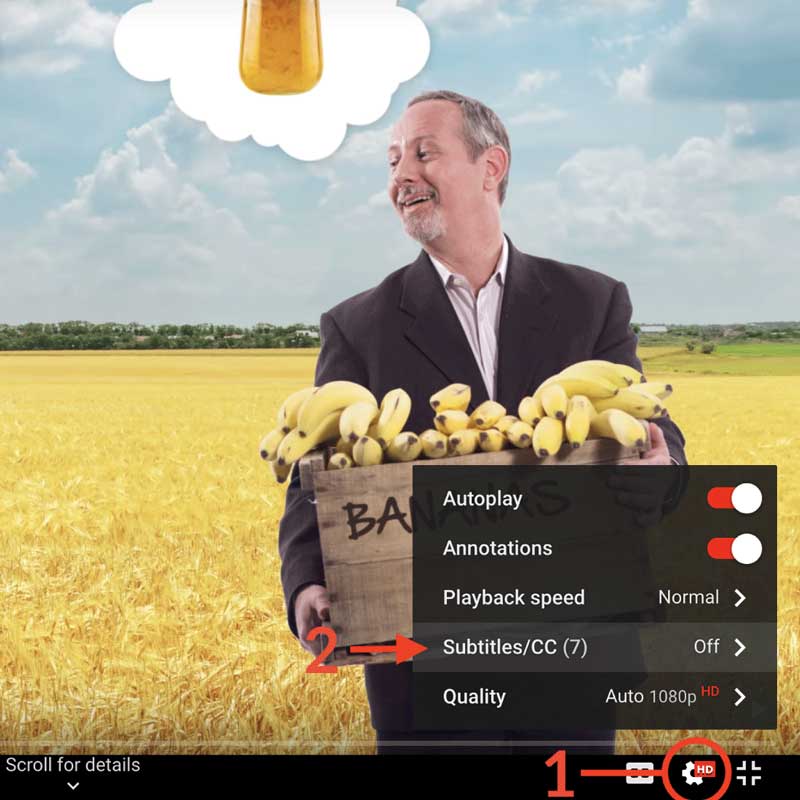
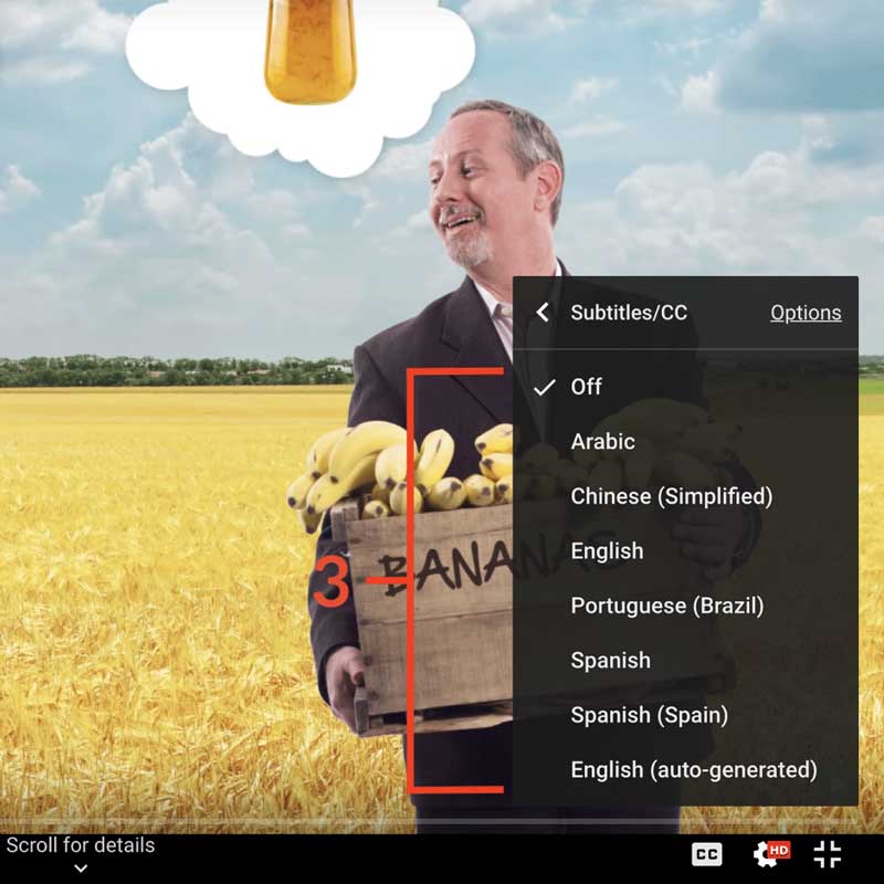
How to turn on captions and select a language:
- Click the settings icon (⚙) at the bottom of the video screen.
- Click Subtitles/CC.
- Select a language.
Contribute Translations!
Join the team and help us provide world-class economics education to everyone, everywhere for free! You can also reach out to us at [email protected] for more info.
Submit subtitles
Accessibility
We aim to make our content accessible to users around the world with varying needs and circumstances.
Currently we provide:
- A website built to the W3C Web Accessibility standards
- Subtitles and transcripts for our most popular content
- Video files for download
Are we missing something? Please let us know at [email protected]
Creative Commons

This work is licensed under a Creative Commons Attribution-NoDerivatives 4.0 International License.
The third party material as seen in this video is subject to third party copyright and is used here pursuant
to the fair use doctrine as stipulated in Section 107 of the Copyright Act. We grant no rights and make no
warranties with regard to the third party material depicted in the video and your use of this video may
require additional clearances and licenses. We advise consulting with clearance counsel before relying
on the fair use doctrine.